Quickstart to ML with dabl
Let’s dive right in!
Let’s start with the classic. You have the titanic.csv file and want to predict whether a passenger survived or not based on the information about the passenger in that file. We know, for tabular data like this, pandas is our friend. Clearly we need to start with loading our data:
>>> import pandas as pd
>>> import dabl
>>> titanic = pd.read_csv(dabl.datasets.data_path("titanic.csv"))
Let’s familiarize ourself with the data a bit; what’s the shape, what are the columns, what do they look like?
>>> titanic.shape
(1309, 14)
>>> titanic.head()
   pclass  survived  ... body                        home.dest
0       1         1  ...    ?                     St Louis, MO
1       1         1  ...    ?  Montreal, PQ / Chesterville, ON
2       1         0  ...    ?  Montreal, PQ / Chesterville, ON
3       1         0  ...  135  Montreal, PQ / Chesterville, ON
4       1         0  ...    ?  Montreal, PQ / Chesterville, ON

[5 rows x 14 columns]
So far so good! There’s already a bunch of things going on in the data that we can see here, but let’s ask dabl what it thinks by cleaning up the data:
>>> titanic_clean = dabl.clean(titanic, verbose=0)
This provides us with lots of information about what is happening in the different columns. In this case, we might have been able to figure this out quickly from the call to head, but in larger datasets this might be a bit tricky. For example we can see that there are several dirty columns with “?” in it. This is probably a marker for a missing value and we could go back and fix our parsing of the CSV, but let’s try and continue with what dabl is doing automatically for now. In dabl, we can also get a best guess of the column types in a convenient format:
>>> types = dabl.detect_types(titanic_clean)
>>> print(types)
                      continuous  dirty_float  ...  free_string  useless
pclass                     False        False  ...        False    False
survived                   False        False  ...        False    False
name                       False        False  ...         True    False
sex                        False        False  ...        False    False
sibsp                      False        False  ...        False    False
parch                      False        False  ...        False    False
ticket                     False        False  ...         True    False
cabin                      False        False  ...         True    False
embarked                   False        False  ...        False    False
boat                       False        False  ...        False    False
home.dest                  False        False  ...         True    False
age_?                      False        False  ...        False    False
age_dabl_continuous         True        False  ...        False    False
fare_?                     False        False  ...        False     True
fare_dabl_continuous        True        False  ...        False    False
body_?                     False        False  ...        False    False
body_dabl_continuous        True        False  ...        False    False

[17 rows x 7 columns]
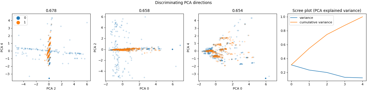
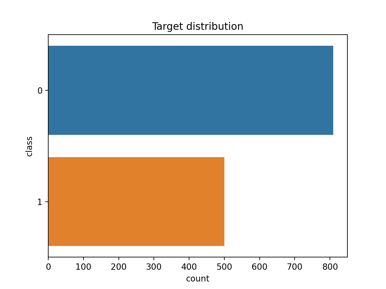
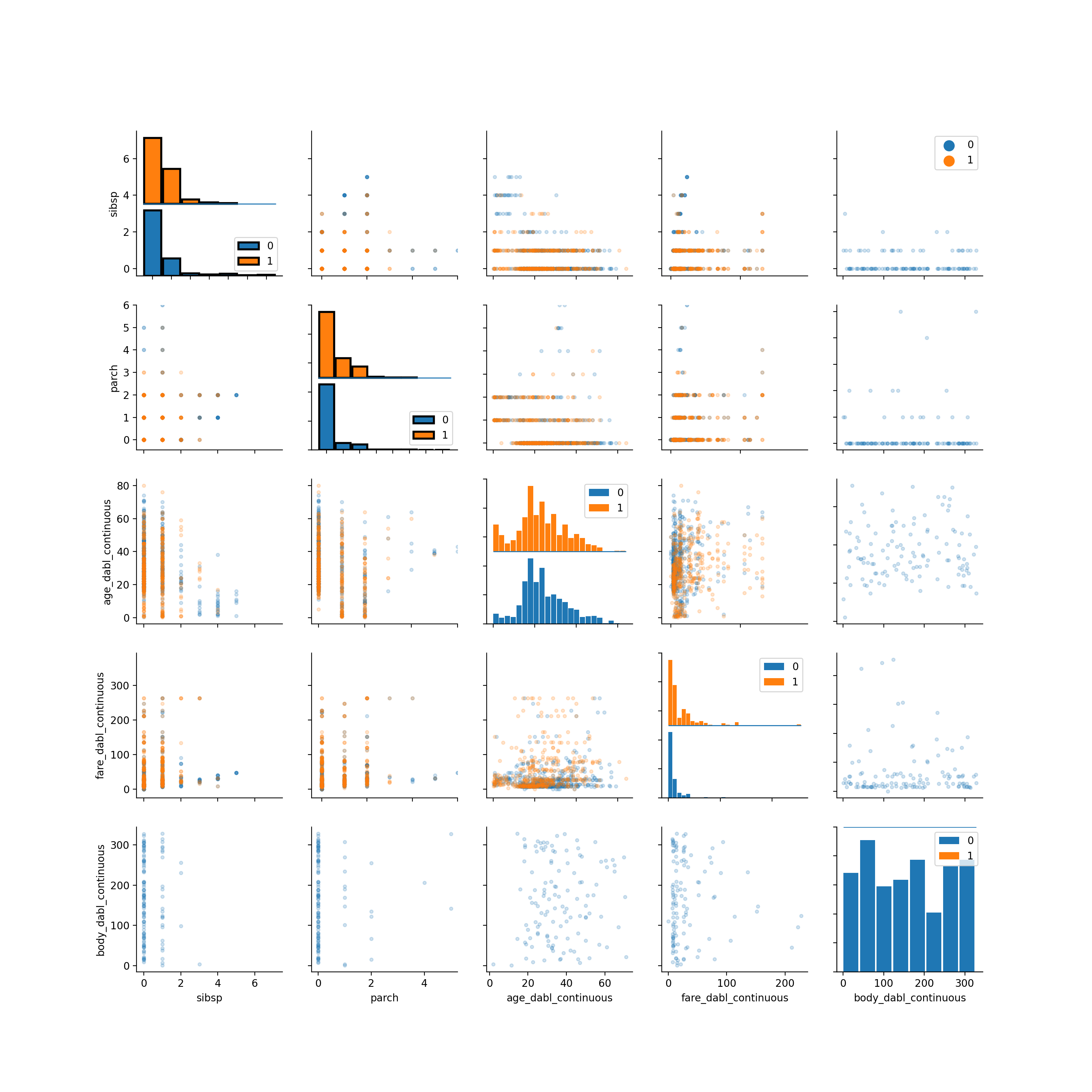
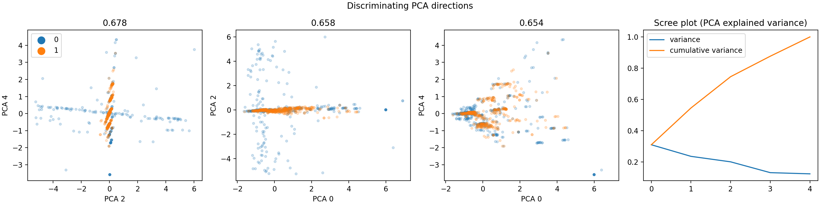
Having a very rough idea of the shape of our data, we can now start looking at the actual content. The easiest way to do that is using visualization of univariate and bivariate patterns. With plot, we can create plot of the features deemed most important for our task.
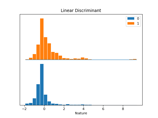
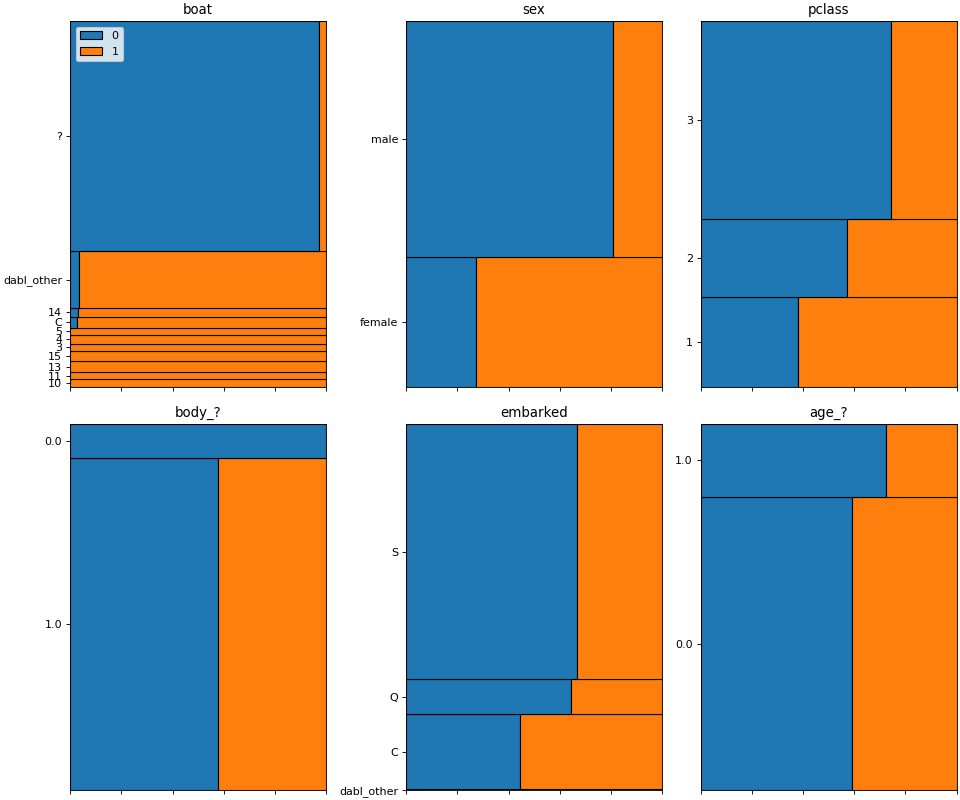
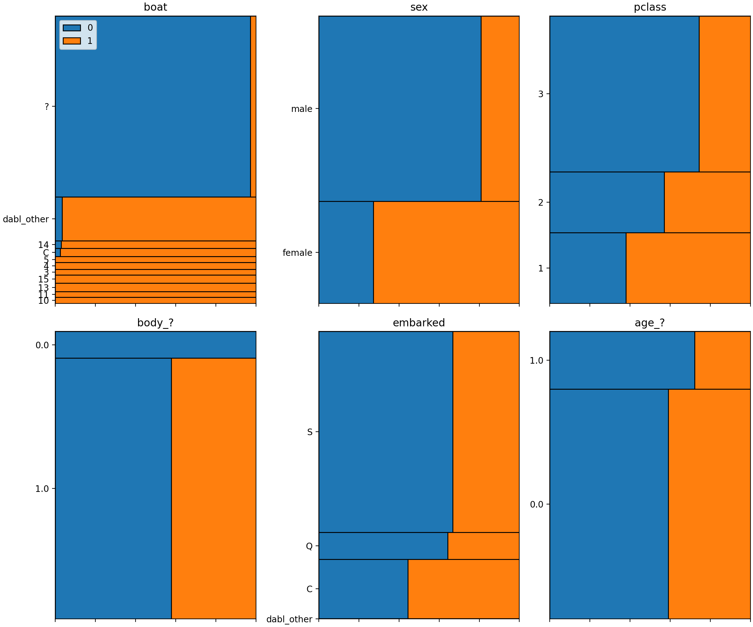
>>> dabl.plot(titanic, 'survived')
Target looks like classification
Linear Discriminant Analysis training set score: 0.578


Finally, we can find an initial model for our data. The SimpleClassifier does all the work for us. It implements the familiar scikit-learn API of fit and predict. Alternatively we could also use the same interface as before and pass the whole data frame and specify the target column.
>>> fc = dabl.SimpleClassifier(random_state=0)
>>> X = titanic_clean.drop("survived", axis=1)
>>> y = titanic_clean.survived
>>> fc.fit(X, y)
DummyClassifier(strategy='prior')
accuracy: 0.618    average_precision: 0.382    recall_macro: 0.500    roc_auc: 0.500
new best (using recall_macro):
accuracy             0.618
average_precision    0.382
recall_macro         0.500
roc_auc              0.500
Name: DummyClassifier(strategy='prior'), dtype: float64
GaussianNB()
accuracy: 0.897    average_precision: 0.870    recall_macro: 0.902    roc_auc: 0.919
new best (using recall_macro):
accuracy             0.897
average_precision    0.870
recall_macro         0.902
roc_auc              0.919
Name: GaussianNB(), dtype: float64
MultinomialNB()
accuracy: 0.888    average_precision: 0.981    recall_macro: 0.891    roc_auc: 0.985
DecisionTreeClassifier(class_weight='balanced', max_depth=1)
accuracy: 0.976    average_precision: 0.954    recall_macro: 0.971    roc_auc: 0.971
new best (using recall_macro):
accuracy             0.976
average_precision    0.954
recall_macro         0.971
roc_auc              0.971
Name: DecisionTreeClassifier(class_weight='balanced', max_depth=1), dtype: float64
DecisionTreeClassifier(class_weight='balanced', max_depth=5)
accuracy: 0.957    average_precision: 0.943    recall_macro: 0.953    roc_auc: 0.970
DecisionTreeClassifier(class_weight='balanced', min_impurity_decrease=0.01)
accuracy: 0.976    average_precision: 0.954    recall_macro: 0.971    roc_auc: 0.971
LogisticRegression(C=0.1, class_weight='balanced')
accuracy: 0.963    average_precision: 0.986    recall_macro: 0.961    roc_auc: 0.989
Best model:
DecisionTreeClassifier(class_weight='balanced', max_depth=1)
Best Scores:
accuracy             0.976
average_precision    0.954
recall_macro         0.971
roc_auc              0.971
Name: DecisionTreeClassifier(class_weight='balanced', max_depth=1), dtype: float64
SimpleClassifier(random_state=0, refit=True, verbose=1)